CHIP data

that plos compu bio under the TF folder
Agius, P., Arvey, A., Chang, W., Noble, W. S., & Leslie, C. (2010). High resolution models of transcription factor-DNA affinities improve in vitro and in vivo binding predictions. PLoS Comput Biol, 6(9). doi: 10.1371/journal.pcbi.1000916

http://www.mskcc.org/research/lab/christina-leslie

http://cbio.mskcc.org/~agiusp/

Accurately modeling the DNA sequence preferences of transcription factors (TFs), and using these models to predict in vivo genomic binding sites for TFs, are key pieces in deciphering the regulatory code. These efforts have been frustrated by the limited availability and accuracy of TF binding site motifs, usually represented as position-specific scoring matrices (PSSMs), which may match large numbers of sites and produce an unreliable list of target genes. Recently, protein binding microarray (PBM) experiments have emerged as a new source of high resolution data on in vitro TF binding specificities. PBM data has been analyzed either by estimating PSSMs or via rank statistics on probe intensities, so that individual sequence patterns are assigned enrichment scores (E-scores). This representation is informative but unwieldy because every TF is assigned a list of thousands of scored sequence patterns. Meanwhile, high-resolution in vivo TF occupancy data from ChIP-seq experiments is also increasingly available. We have developed a flexible discriminative framework for learning TF binding preferences from high resolution in vitro and in vivo data. We first trained support vector regression (SVR) models on PBM data to learn the mapping from probe sequences to binding intensities. We used a novel -mer based string kernel called the di-mismatch kernel to represent probe sequence similarities. The SVR models are more compact than E-scores, more expressive than PSSMs, and can be readily used to scan genomics regions to predict in vivo occupancy. Using a large data set of yeast and mouse TFs, we found that our SVR models can better predict probe intensity than the E-score method or PBM-derived PSSMs. Moreover, by using SVRs to score yeast, mouse, and human genomic regions, we were better able to predict genomic occupancy as measured by ChIP-chip and ChIP-seq experiments. Finally, we found that by training kernel-based models directly on ChIP-seq data, we greatly improved in vivo occupancy prediction, and by comparing a TF's in vitro and in vivo models, we could identify cofactors and disambiguate direct and indirect binding.

Transcription factors (TFs) are proteins that bind sites in the non-coding DNA and regulate the expression of targeted genes. Being able to predict the genome-wide binding locations of TFs is an important step in deciphering gene regulatory networks. Historically, there was very limited experimental data on the DNA-binding preferences of most TFs. Computational biologists used known sites to estimate simple binding site motifs, called position-specific scoring matrices, and scan the genome for additional potential binding locations, but this approach often led to many false positive predictions. Here we introduce a machine learning approach to leverage new high resolution data on the binding preferences of TFs, namely, protein binding microarray (PBM) experiments which measure the in vitro binding affinities of TFs with respect to an array of double-stranded DNA probes, and chromatin immunoprecipitation experiments followed by next generation sequencing (ChIP-seq) which measure in vivo genome-wide binding of TFs in a given cell type. We show that by training statistical models on high resolution PBM and ChIP-seq data, we can more accurately represent the subtle DNA binding preferences of TFs and predict their genome-wide binding locations. These results will enable advances in the computational analysis of transcriptional regulation in mammalian genomes.

Trained SVRs yield more accurate in vitro TF binding models

We first tested the performance of our SVR models on in vitro binding preferences, in order to establish that they could better capture TF sequence specificities than existing approaches. For 33 yeast and 114 mouse TFs, experimental data for two independent PBM array designs were available [9], [10], measuring TF binding against two completely disjoint PBM probe sets. This combined data set provided a perfect cross-validation setting where we trained a model using data from one array design (“training PBM”) and then tested the model's ability to predict binding preferences on the other array design's probe sequences (“test PBM”). We benchmarked the SVR models against the E-score approach [3], using the E-scores for all 8-mer patterns, both contiguous and gappy, as computed and posted on the Uniprobe database[11]. E-scores are modified Wilcoxon rank statistics that assess the enrichment of a given 8-mer sequence pattern in probe sequences at the top of the intensity ranking in a PBM experiment. These scores range from −0.5 to 0.5, where scores approaching 0.5 indicate that the 8-mer pattern is mostly present in bound probe sequences. In their yeast in vivopredictions, [9] identify high scoring 8-mer patterns to predict TF binding preferences. Therefore, we compared SVR performance to a maximum E-score approach, where each probe sequence in the test PBM is assigned the maximal E-score over the 8-mer patterns it contains, and the E-scores are computed on the training PBM. We call this the E-max score. We note that due to feature selection, our models contain no more than 4,000 -mer features. By contrast, for the data set 114 mouse TFs, the average number of -mers with E-scores above 0.35 (the threshold used for reporting the pattern) was 13,300, with just 10 of the TFs having fewer than 3,000 -mers and 64 having more than 10,000 -mers. In this sense, the SVR models are more compact than the E-score approach.

Figure 5. Sequence feature analysis of in vitro and in vivo models.

ChIP-derived SVMs capture information about cofactor motifs

We next performed a similar feature analysis of the ChIP-derived model for Sox2, one of the examples where the in vivo model strongly outperformed the in vitro model. Here, 13-mer features from the SVM model are represented by their vector of alignment scores relative to 60bp sequences under ChIP-seq peaks rather than probe sequences.

Again, we identified two well-separated clusters, shown using stars and circles in Figure 5(b). Here, the cluster representative for the “star” cluster can be expanded to a PSSM that closely resembles the Sox2 motif. However, the representative for the “circle” cluster maps to part of the Oct4 octamer motif, indicating that the ChIP-derived model is learning binding information about Sox2's binding partner Oct4 (Figure 5(c)). We hypothesized that this additional cisinformation may account for part of the improvement of the in vivo model over the PBM-derived model. To quantify this effect, we identified Sox2 bound regions that are not detected by the PBM-trained SVR model but are correctly detected by the ChIP-trained SVM (Figure S9(a) inText S1). These 33 60bp regions were 6-fold depleted for the core Sox2 motif TTGT and 3-fold enriched for the core Oct4 motif TGCA. Moreover, 32 out of 33 of these regions were detected as positives by the PBM-trained SVR for Oct4 (). These results suggest that some binding of Sox2 may be indirect via binding of the cofactor Oct4.

Discussion

Overview of SVR training

We developed a training strategy for our SVR models that involved three key components: (1) the choice of kernel, which specifies the space of features used to compare pairs of probe sequences; (2) the sampling procedure for selecting the training sequences, which produces more informative training data and reduces training time; (3) the feature selection method, which eliminates unimportant features and further improves computational efficiency. Each component is described in more technical detail below. We used the LIBSVM package for the computation of SVR models, keeping the  parameter fixed at 0.1 for all experiments.

The di-mismatch kernel

Training a kernel method like an SVR on sequence data requires the use of some kind of string kernel, i.e. a similarity measure between sequences that defines an inner product in a corresponding feature space. Various -mer based string kernels have been proposed, including the  mismatch kernel [5], where the feature representation for a sequence amounts to an inexact-matching histogram of -mer counts, allowing up to  mismatches in each -mer match (). Here, however, even for small values of the mismatch parameter, this kernel tends to make the “mismatch” neighborhood of a given -mer too large.

We therefore developed a novel first order Markov mismatch kernel, called the di-mismatch kernel, that counts mismatching dinucleotides and that inherently favors -mers with consecutive mismatches. Let  be a set of unique -mers that occur in the set of training sequences (PBM probe sequences). Given a training sequence  of length , we define the set of substrings of length  in  to be
Then  may be represented by the feature vector
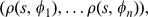
where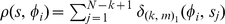 , and the value  is the di-mismatch score between two -mers, which counts the number of matching dinucleotides between and , that number being set to zero if this count falls below the threshold , where  is the maximum number of mismatches allowed.

This score inherently favors consecutive mismatches, as we show in the following examples. Consider the first pair of 13-mers shown with four non-consecutive mismatches, which results in 6 mismatching dinucleotides out of 12: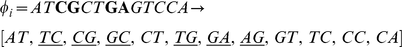

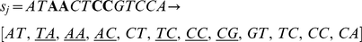
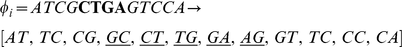
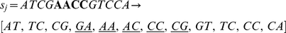
In contrast, the following pair of 13-mers with four consecutive mismatches leads to a count of 5 mismatching dinucleotides.

By enforcing a mismatch parameter of , we induce sparsity in the feature counts and seem to obtain more meaningful “neighborhoods” of the features  than the standard mismatch kernel. This procedure appeared to capture the full dynamic range of effective binding while downsampling the large number of unbound probes.

Since the PBM arrays are designed to give good coverage of 8-mer patterns (including gapped patterns), we chose  parameters that would require at least 8 matching characters between the -mers. Our parameter experiments on one set of yeast PBM arrays [9] indicated  to be the best parameter setting, and we used this kernel choice for the in vitro evaluation for most of our reported results. However, one may use a 10-fold cross-validation approach on the training PBM array to perform a grid-search and thereby optimize the choice of the  parameters. We used such a strategy for the 7 mammalian in vivooccupancy predictions (Figure 4), whereby we tested  parameters ranging from  and  where .

Much like the mismatch kernel, the computational cost of scoring test sequences with the trained di-mismatch SVM/SVR model is linear with respect to the input sequence length. Every-mer has a non-zero match score to a fixed number of features, and each feature is represented by a weight in the support vector model. Therefore, the contribution of each -mer can be pre-computed, and those with non-zero contribution can be stored in a hash table.

Sampling PBM data to obtain an informative training set

Standard PBM arrays typically contain 44K probes, each associated with a binding intensity score, but only few hundred probes indicate some level of TF binding. Using all of the PBM probes as training data would allow the SVR to achieve good training loss simply by learning that most probes have low binding scores. In order to learn sequence information associated with the bound probes, we selected training sequences from the tails of the distribution of the normalized binding intensities. More specifically, we selected the set of “positive” training probes to be those sequences associated with normalized binding intensities ; if the number of such probes was less than 500, we selected the top 500 probes ranked by their binding signals. The same number of “negative” training probes was selected from the other end of the distribution. This procedure appeared to capture the full dynamic range of effective binding for learning the regression model while downsampling the large number of unbound probes. We also tried sampling “negative” probes from the full intensity distribution (anywhere outside the positive tail), but we found that using the negative tail yielded better results.

Feature selection

Careful feature selection can eliminate noisy features and of course reduces computational costs, both in the training and testing of the model. In particular, choosing very infrequent -mers may add noise, and ideally, sequence features should display a preference either for bound or unbound probes. Therefore, we selected the feature set  to be those -mers that are over-represented either in the “positive” or “negative” probe class by computing the mean di-mismatch score for each -mer in each class and ranking features by the difference between these means. In all reported results, we used at most 4000 -mers for our models.

ChIP-seq processing

We processed the ChIP-seq data using the SPP package [21] and extracted the top 1000 peaks to define a gold standard for occupancy. A 60bp window was selected around each of the peaks and used as the positive examples. A 60bp window 300bp to the left of the peak was selected as the negative example.

Extracting features from SVR/SVM models

It is informative to be able to use the SVM model to visualize the -mers that contribute to the model. Here our goal is to visually represent both (i) the similarity of -mer features based on their support across the training data representing and (ii) the contribution (or weight) of these -mers to the model.

To obtain a similarity measure between -mer features extracted from the trained models, we represented each -mer by a vector of alignment scores against the positive training sequences used to compute the SVR model: we found the optimal ungapped alignment of the -mer to each training sequence and used the number of match positions as the alignment score. Intuitively, sequence-similar -mers will have similar alignment scores across the training examples, so they will be represented by nearby vectors in this representation. However, we are not explicitly modeling sequence dependence but instead relying on co-occurrence of matches of similar -mers. We then performed -means clustering ( = 2) on the vectors representing the 13-mer features. Next we used the SVM/SVR weight vector , derived from the solution to the optimization problem, to select the top 500 representatives for each cluster, thereby reducing the rest of our analysis to -mers that contributed significantly to the model. Next, we projected the 1000 -mers to a two-dimensional representation using principal component analysis (PCA), distinguishing cluster members with circles and stars in the plot. The relative significance of each feature is indicated by a color scale ranging from red to blue, for high and low  respectively.

Finally, we defined a cluster representative for each group by the feature that has the following two properties: (i) it is in the top quartile of the  weights for that cluster, and (ii) it is the closest feature to the cluster centroid. This gives us a cluster representative that is simultaneously close to the true cluster centroid and significant for the model. Finally, to represent a given -mer feature by a motif logo, we selected the top 50 positive training sequences that best aligned with the -mer, extracted the -length sequences that matched the feature, and computed a PSSM.